Backtrader Tutorial: Build & Backtest Algorithmic Trading Strategies

Backtrader is a Python framework designed for creating and backtesting trading strategies. It simplifies the process by providing tools like the Cerebro engine to integrate data feeds, strategies, and analyzers. The platform supports historical data, live trading integrations, and over 122 built-in indicators. Here's what you'll learn:

• Installation: Install Backtrader and optional libraries for charting or broker connections.
• Setup: Configure the Cerebro engine, broker settings, and load historical data.
• Strategy Creation: Build a Moving Average Crossover strategy to identify buy/sell signals.
• Backtesting: Run simulations to evaluate strategy performance with visual outputs.
• Optimization: Fine-tune parameters like moving average periods for better results.
• Risk Management: Implement position sizing and set stop-loss/take-profit levels.

Whether you're new to algorithmic trading or looking to improve your strategies, Backtrader provides a user-friendly way to test and refine your ideas. Let's dive into the details.

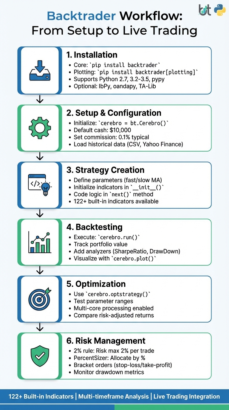
Backtrader Workflow: 6-Step Guide to Building and Testing Trading Strategies

Setting Up Backtrader: Installation and Configuration

Installing Backtrader and Dependencies

Getting started with Backtrader is straightforward. Start by installing the core library. Open your terminal and run:

pip install backtrader

This command takes care of the main backtesting library. If you want to enable charting, you'll need Matplotlib. Use:

pip install backtrader[plotting]

This ensures Matplotlib (version 1.4.1 or higher) and its required dependencies are installed. Keep in mind that while Backtrader supports Python 2.7, 3.2 through 3.5, and pypy/pypy3, plotting won't work on pypy environments because Matplotlib isn't compatible there.

For those looking to connect with live brokers, additional libraries are necessary:

• Interactive Brokers: Install IbPy from GitHub (not PyPI) and include pytz for timezone management.
• Oanda: Use the oandapy library.
• Visual Chart: This requires a specific comtypes fork alongside pytz.
• TA-Lib Indicators: Install the Python ta-lib wrapper separately if you plan to use these indicators. While Backtrader includes over 122 built-in indicators, TA-Lib offers additional options.

Once you've completed the installation, you can move on to configuring the environment, starting with Cerebro and broker settings.

Configuring Cerebro and Broker Settings

With Backtrader installed, you can initialize the Cerebro engine by running:

cerebro = bt.Cerebro()

This engine serves as the backbone of your backtesting setup, combining data feeds, strategies, and analyzers. By default, the built-in broker starts with a cash balance of $10,000.00, but you can customize this to fit your trading capital. For example:

cerebro.broker.setcash(100000.0)

To make your backtests more realistic, you'll want to account for commission fees. Set these with:

cerebro.broker.setcommission(commission=0.001)

Here, 0.001 represents a 0.1% fee per trade, which is fairly standard for many brokers. You can also check your portfolio value at any point during the backtest using:

cerebro.broker.getvalue()

For executing orders at the opening price of the current bar, enable:

cheat_on_open=True
cerebro.broker.set_coo(True)

To optimize performance, Cerebro preloads data feeds (preload=True) and processes indicators in vectorized mode (runonce=True). If you prefer cleaner charts, you can disable default observers with:

stdstats=False

With these settings in place, you're ready to load historical data.

Loading Historical Data

Backtrader supports a variety of data formats, including Yahoo Finance CSV files, VisualChart, and generic CSV files. If you're using Yahoo Finance data stored locally, create a data feed with:

bt.feeds.YahooFinanceCSVData

For files with dates in descending order, simply add reverse=True when initializing the feed.

For custom CSV files, use:

bt.feeds.GenericCSVData

Here, you'll map each column in the file to its corresponding field (e.g., datetime, open, high, low, close, volume, and open interest). Specify the format of your date strings with the dtformat parameter. For example:

• %Y-%m-%d for dates like 2026-02-15
• %m/%d/%Y for dates like 02/15/2026

Adjust the separator parameter to match your file's delimiter, whether it's a comma, tab, or semicolon.

After setting up your data feed, add it to Cerebro:

cerebro.adddata(data)

You can narrow down the backtest to specific periods using the fromdate and todate parameters. If your CSV contains missing values, use the nullvalue parameter to replace them with 0.0 or float('NaN'). For repeated custom formats, consider subclassing GenericCSVData and predefining the parameters.

With historical data loaded and configured, you're ready to start running your backtests.

Building a Moving Average Crossover Strategy

How the Moving Average Crossover Works

A moving average crossover strategy relies on plotting two types of moving averages: a "fast" moving average with a shorter time frame and a "slow" moving average with a longer time frame. The basic rule is simple: buy when the fast moving average crosses above the slow one, and sell or exit when it crosses below.

"The crossover strategy works by plotting two moving averages – one with a shorter time frame (i.e., the 'fast' MA) and one with a longer time frame (i.e., the 'slow' MA). This strategy is based on the idea that short-term price movements are more volatile than long-term price movements." - Nate B, Author and Trader

"The crossover strategy works by plotting two moving averages – one with a shorter time frame (i.e., the 'fast' MA) and one with a longer time frame (i.e., the 'slow' MA). This strategy is based on the idea that short-term price movements are more volatile than long-term price movements." - Nate B, Author and Trader

This method is favored by many traders because it's straightforward to grasp, easy to execute, and allows flexibility in adjusting time frames to match individual trading preferences.

For example, in January 2023, trader Nate B shared a backtest of a Moving Average Crossover strategy using Backtrader on the SPY ticker. Starting with $100,000 on January 1, 2022, the strategy executed six trades over the year and closed on December 31, 2022, with a profit of $978.24. This performance outshined a simple buy-and-hold approach for the same asset, which would have resulted in a loss of nearly 20% ($19,945.15) during the same period.

Let’s explore how you can implement this strategy using Backtrader.

Coding the Strategy in Backtrader

To implement the Moving Average Crossover strategy in Backtrader, you’ll start by defining a class that inherits from bt.Strategy. This allows you to set up adjustable parameters for the moving averages:

class SmaCross(bt.Strategy):
    params = (
        ('pfast', 10),
        ('pslow', 30),
    )

Within the __init__() method, you’ll declare the indicators. This is where Backtrader calculates the moving averages before the backtest begins:

def __init__(self):
    sma1 = bt.ind.SMA(period=self.p.pfast)
    sma2 = bt.ind.SMA(period=self.p.pslow)
    self.crossover = bt.ind.CrossOver(sma1, sma2)

The bt.ind.CrossOver indicator simplifies the logic by returning 1.0 when the fast moving average crosses above the slow one, and -1.0 when it crosses below.

Next, you’ll write the trading logic in the next() method, which processes each new data bar:

def next(self):
    if not self.position:
        if self.crossover > 0:
            self.buy()
    elif self.crossover < 0:
        self.close()

Here’s how it works:

• The if not self.position condition ensures that only one position is active at a time.
• When the crossover is positive (fast MA crosses above slow MA) and there’s no current position, the strategy enters a long position by buying.
• If a position is already active and the crossover turns negative (fast MA crosses below slow MA), the strategy exits by closing the position.

Keep in mind that the strategy only starts executing after enough data bars have been processed to calculate the moving averages (in this case, 30 bars). This ensures the indicators are fully initialized before any trades occur.

Running Backtests and Analyzing Results

Executing the Backtest

Once you've coded your strategy, running a backtest becomes a straightforward process. The cerebro.run() method handles the simulation and returns a list of strategy instances created during the run. After execution, you can access indicators, observers, and analyzers for detailed insights.

Here’s a simple example of how to execute a backtest:

cerebro = bt.Cerebro()
cerebro.adddata(data)
cerebro.addstrategy(SmaCross)
cerebro.broker.setcash(100000.0)

print(f'Starting Portfolio Value: ${cerebro.broker.getvalue():,.2f}')
results = cerebro.run()
print(f'Final Portfolio Value: ${cerebro.broker.getvalue():,.2f}')

The cerebro.broker.getvalue() method provides the portfolio's total value at any given point. You can adjust the initial cash value to suit your testing needs.

For more detailed performance metrics, you can add analyzers before running the backtest. For instance, the SharpeRatio analyzer evaluates risk-adjusted returns:

cerebro.addanalyzer(bt.analyzers.SharpeRatio, _name='sharpe')
results = cerebro.run()
sharpe_value = results[0].analyzers.sharpe.get_analysis()
print(f'Sharpe Ratio: {sharpe_value}')

Once the simulation is complete, you can visualize the strategy's performance using Backtrader's built-in charting tools.

Creating Performance Charts

To better understand your strategy's performance, Backtrader offers a simple way to generate charts through the cerebro.plot() method. These charts, created using matplotlib, display price data, indicators, and trade execution points, giving a clear picture of your strategy's behavior during the backtest.

cerebro.plot()

By default, the plot includes three Standard Stats observers:

• CashValue: Tracks the cash and total portfolio value over time.
• Trade: Displays the profit or loss from closed trades.
• BuySell: Marks the buy and sell execution points on the price chart.

If the chart appears too cluttered, you can use the numfigs parameter to split the view into multiple figures for better clarity. Alternatively, disable the default observers by setting stdstats=False when running the backtest:

cerebro.run(stdstats=False)

"This class [Cerebro] is the cornerstone of backtrader because it serves as a central point for: Gathering all inputs (Data Feeds), actors (Strategies), spectators (Observers), critics (Analyzers) and documenters (Writers)... Execute the backtesting/or live data feeding/trading." - Backtrader Documentation

"This class [Cerebro] is the cornerstone of backtrader because it serves as a central point for: Gathering all inputs (Data Feeds), actors (Strategies), spectators (Observers), critics (Analyzers) and documenters (Writers)... Execute the backtesting/or live data feeding/trading." - Backtrader Documentation

The visualizations are especially helpful for spotting patterns like drawdown periods or trade frequency, giving you actionable insights to refine your strategy before diving into optimization.

Optimizing Strategy Parameters

Defining Parameter Ranges

After completing backtesting, the next step is to fine-tune your strategy's parameters for better performance. In Backtrader, you can use cerebro.optstrategy() to test multiple parameter combinations by running several instances of your strategy.

Parameters should be passed as iterables, such as ranges, lists, or tuples. For sequential values like moving average periods, Python's range() function works perfectly:

cerebro.optstrategy(SmaCross, pfast=range(10, 31), pslow=range(30, 51))

If the values are not sequential, you can use a list or tuple instead:

pfast=[10, 15, 20, 25]

To speed up optimization, Backtrader automatically uses all available CPU cores. If you want to limit this, adjust the maxcpus parameter. Additionally, the optreturn=True option (enabled by default) ensures only key parameters and analyzer results are returned, rather than the full strategy objects. This saves memory and speeds up the process.

Once your parameter combinations are set, you can evaluate their performance using analyzers.

Comparing Optimization Results

When the optimization process is complete, cerebro.run() will return a list of lists. Each inner list corresponds to the strategy instances for one specific parameter combination. Before running the optimization, it’s a good idea to add analyzers like SharpeRatio, DrawDown, or Returns to measure performance:

cerebro.addanalyzer(bt.analyzers.SharpeRatio, _name='sharpe')
cerebro.addanalyzer(bt.analyzers.DrawDown, _name='drawdown')
results = cerebro.run()

You can then extract performance metrics by looping through the results and accessing the analyzers:

for result in results:
    strat = result[0]
    sharpe = strat.analyzers.sharpe.get_analysis()
    drawdown = strat.analyzers.drawdown.get_analysis()
    print(f'Fast: {strat.params.pfast}, Slow: {strat.params.pslow}, Sharpe: {sharpe["sharperatio"]:.2f}')

When evaluating strategies, focus on risk-adjusted returns, such as the Sharpe Ratio, rather than just raw profits. High returns can be tempting, but if they come with significant drawdowns, the strategy might not be suitable for live trading. The Maximum Drawdown metric reveals the largest drop from a peak to a trough, helping you gauge whether you could handle the strategy's rough patches psychologically.

Finally, avoid blindly choosing parameters that performed the best historically. These may simply be overfitted to past data and might not reflect a real trading edge. Always balance performance with robustness to ensure your strategy can handle future market conditions effectively.

Managing Position Size and Risk

Implementing Position Sizing

Backtrader’s default SizerFix trades one unit per order. While simple, it’s not practical for most strategies. Instead, you can use a more flexible sizer to control your position size.

One straightforward way to do this is by using cerebro.addsizer(). For example, to allocate 10% of your available cash per trade, you can add the following:

cerebro.addsizer(bt.sizers.PercentSizer, percents=10)

This method automatically adjusts your position size as your portfolio balance changes. If you start with $10,000 in cash, each trade will use around $1,000. When your account grows to $15,000, the next trade will increase to $1,500.

Another popular approach is the 2% rule, which limits the risk on a single trade to 2% of your total capital. For instance, with $10,000 in capital, a $10.00 entry price, and a $9.00 stop-loss, you would calculate your position size as 200 shares, ensuring your risk is capped at $200.

Here’s the formula:
Position Size = (Total Capital × Risk %) / (Entry Price - Stop Loss Price)

You can integrate this calculation into your strategy’s next() method by using self.broker.get_cash() to determine your available capital and factoring in the stop-loss distance.

Risk Management Best Practices

Position sizing is just one part of managing risk - it’s equally important to protect your capital during trades.

Proper position sizing can shield your portfolio during drawdowns. Even a profitable strategy can fail if you overexpose yourself on a single trade. The 2% rule is a safeguard against this. As Xavier Escudero puts it:

"The 2% rule is a risk management technique in trading... which states that we should not risk more than 2% of our total account capital in a single trade".

"The 2% rule is a risk management technique in trading... which states that we should not risk more than 2% of our total account capital in a single trade".

Don’t forget to account for trading costs when backtesting. Use cerebro.broker.setcommission() to include transaction fees and slippage. Many strategies that look profitable in theory fail in live trading because they ignore these costs.

Backtrader also offers bracket orders (buy_bracket and sell_bracket), which let you attach stop-loss and take-profit orders directly to your entry. This ensures every trade has a defined risk-reward profile. Additionally, you can use order_target_percent() to keep your exposure to a single asset within a specific percentage of your portfolio, reducing the risk of over-concentration.

Finally, always monitor your drawdown during backtesting. Adding the DrawDown observer allows you to visualize peak-to-trough declines in your equity curve. This helps you evaluate whether you can handle the psychological challenges of a strategy’s rough periods before committing real money.

Conclusion

You now have everything you need to create, test, and refine Backtrader strategies. From setting up Cerebro and working with init and next, to running realistic backtests, optimizing parameters, and managing risk, the foundation is in place.

A key takeaway is understanding Backtrader's "Index 0" approach and its Lines concept. Always initialize indicators in init to take advantage of vectorized calculations, which make backtesting faster and more efficient.

Once your backtests are complete, take your analysis further. Use tools like SharpeRatio and Drawdown analyzers to assess risk-adjusted performance beyond just portfolio value. Visualize your results with cerebro.plot() and dive into the official documentation at backtrader.com/docu for advanced features like multi-timeframe analysis, custom order types, and live trading integration with brokers such as Interactive Brokers and Oanda.

Now it’s time to refine your strategies. Start by tweaking your moving average crossover approach. Experiment with different parameter ranges, incorporate commission costs with setcommission(), and fine-tune position sizing. You can also explore bracket orders for automated stop-loss and take-profit levels or use bt.SignalStrategy for declarative trade signals.

Keep iterating and testing. Utilize optstrategy for parameter optimization, monitor orders with notify_order, and account for slippage and transaction costs to ensure realistic performance. With consistent effort, your strategies will be better equipped to handle various market conditions.

FAQs

How do I add slippage to make my Backtrader backtests more realistic?

To incorporate slippage into your Backtrader backtests, you can tweak the broker's slippage settings. For instance, you can use parameters like slip_perc for percentage-based slippage or slip_fixed for a fixed amount.

For example, setting slip_perc=0.005 applies a 0.5% slippage to your trades. Additionally, enabling slip_open ensures slippage is applied at the next bar's opening price. You can also fine-tune settings such as slip_limit for limit orders, allowing for a more realistic simulation of market behavior.

How can I prevent overfitting when using optstrategy for optimization?

When working with optstrategy, it's important to take steps to prevent overfitting. Start by limiting excessive optimization, as over-tweaking can lead to strategies that only work well on specific historical data but fail in real-world scenarios. Use a diverse and extensive set of training data to ensure your strategy is exposed to a wide range of market conditions.

Additionally, factor in transaction costs during your analysis. Ignoring these can result in strategies that look profitable on paper but aren't viable in practice. Finally, focus on strategies that show consistent performance across multiple datasets, rather than those that simply align closely with historical data. This approach builds trading strategies that are more dependable and resilient.

How do I use bracket orders for stop-loss and take-profit in Backtrader?

When using bracket orders in Backtrader, the buy_bracket method simplifies the process of placing a primary order along with linked stop-loss and take-profit orders. For instance, calling self.buy_bracket(limitprice=14.00, stopprice=13.00) creates a buy order at $14.00, with a stop-loss set at $13.00. These orders are submitted simultaneously and are automatically managed. This ensures that the stop-loss and take-profit orders are executed or canceled depending on the status of the main order.