Jump Diffusion Model Explained: Applications in Finance & Trading

The Jump Diffusion Model is a mathematical framework that improves upon standard models like Black-Scholes by accounting for both normal price changes and sudden, unpredictable market shocks. This dual approach makes it particularly useful for pricing options, managing financial risk, and understanding market behaviors like volatility smiles and fat tails.

Key Insights:

• What it is: A model combining continuous price changes (Geometric Brownian Motion) with random jumps (Poisson process).
• Why it matters: Standard models fail to explain abrupt price changes or extreme risks, leading to inaccurate pricing and risk assessments.
• Applications: Pricing exotic options, managing Value-at-Risk (VaR), and developing trading strategies for volatile markets.

How It Works:

• Formula: dSₜ = μ Sₜ dt + σ Sₜ dWₜ + (J – 1) Sₜ dN(t)
  • Drift (μ): Expected return.
  • Diffusion (σ): Day-to-day price changes.
  • Jump (λ, m, ν): Frequency, size, and volatility of jumps.

By incorporating jumps, the model better reflects market realities, making it a go-to for traders, quants, and risk managers dealing with turbulent conditions.

Core Mechanics of the Jump Diffusion Model

How the Jump Diffusion Model Works

The Jump Diffusion Model builds upon the Black-Scholes framework by introducing a jump component to the Geometric Brownian Motion. Its behavior is described by the stochastic differential equation:

dSₜ = μ Sₜ dt + σ Sₜ dWₜ + (J – 1) Sₜ dN(t)

Here’s how it breaks down:

• The first term (μ Sₜ dt) represents the drift, which accounts for the asset's expected return over time.
• The second term (σ Sₜ dWₜ) models the diffusion, capturing the typical daily price fluctuations.
• The third term ((J – 1) Sₜ dN(t)) introduces the jump process, where jumps occur randomly, altering the asset price by a factor of J when they happen.

This jump component is driven by a Poisson process, meaning jumps occur at unpredictable times, disrupting the otherwise continuous price path. These instantaneous changes in value create "market incompleteness" because they cannot be perfectly hedged.

"If we relax the assumption of GBM and introduce the concept of discontinuous jumps in the stock price then it becomes impossible to perfectly hedge and leads to market incompleteness." - QuantStart

The inclusion of jumps transforms the Black-Scholes partial differential equation (PDE) into a partial integro-differential equation (PIDE), better capturing real-world market shocks. To fully grasp the model, it's essential to understand its parameters and their financial interpretations.

Key Parameters and Their Financial Meaning

Each parameter in the Jump Diffusion Model connects directly to observable market behaviors:

Parameter	Symbol	Financial Meaning
Drift	μ	Represents the expected annual return, or the asset's long-term trend.
Diffusion Volatility	σ	Reflects the typical day-to-day price changes.
Jump Intensity	λ	Indicates the average number of jumps per year, often linked to events like earnings announcements or geopolitical shocks.
Mean Jump Size	m	Represents the average effect a jump has on the asset price.
Jump Volatility	ν	Captures the uncertainty in the size of each jump.

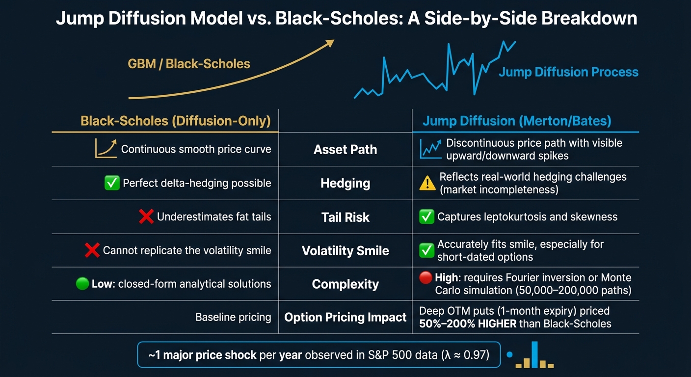
For example, when analyzing S&P 500 data from January 2021, the jump intensity (λ) was approximately 0.97. This suggests about one major price shock per year on average. Merton's approach to modeling jump size assumes that the logarithm of J follows a normal distribution, allowing for both upward and downward price shifts.

By understanding these parameters, we can delve into different model variants tailored to reflect diverse market scenarios.

Common Variants of the Jump Diffusion Model

Over time, several adaptations of the Jump Diffusion Model have been developed to address specific market dynamics:

• Merton's Jump Diffusion Model (1976): This classic version provides a semi-closed form solution for option pricing, expressed as a weighted sum of Black-Scholes prices for varying numbers of jumps.
• Kou's Double Exponential Model: This variation uses a double-exponential distribution for jump sizes, better capturing the heavy tails and volatility skew seen in real market data.
• Lévy-driven Extensions: Models like the Variance Gamma and Normal Inverse Gaussian expand the jump process, offering a more nuanced view of tail behavior and jump frequency.

In specialized applications, such as interest rate or credit risk modeling, Affine Jump Diffusion models are often employed. Meanwhile, ARCH/GARCH Jump Diffusion hybrids incorporate time-dependent volatility into the jump process, making them particularly useful for equity markets. These variants allow the model to adapt to a wide range of financial scenarios.

How to Implement the Jump Diffusion Model

Data Requirements and Preprocessing

To effectively implement the jump diffusion model, you'll need two main types of data: historical time-series data and option market data. Historical data, ideally daily or high-frequency, helps estimate physical parameters. Meanwhile, option market data - covering strikes, bid/ask prices, and maturities - provides the foundation for risk-neutral calibration.

Before diving into estimation, transform raw asset prices into logarithmic returns using $X_t = \ln(S_t/S_0)$. This step ensures the data aligns with the stochastic differential equations used in the Merton and Kou models. For option calibration, calculate the midpoint of bid and ask prices ($(Bid + Ask) / 2$). This approach reduces the noise caused by bid-ask spreads, giving you a cleaner dataset for calibration.

Calibration and Estimation Methods

Once your data is ready, the next step is calibrating the model parameters. The most widely used method for this is Maximum Likelihood Estimation (MLE), which requires a well-defined transition density. The COS method is often applied here to compute this density. Alternatively, the Generalized Method of Moments (GMM) offers a simpler path by working directly with the empirical characteristic function, bypassing the need for a density function.

When estimating the diffusion volatility ($\sigma$) and jump intensity ($\lambda$), always do so jointly. Estimating them separately can introduce bias since both components influence the noise in small returns.

For calibrating live market option prices, a least-squares objective function is a practical choice. Using Python's scipy.optimize.minimize with the SLSQP method, you can fit model prices to observed midpoint prices across various strikes. To ensure meaningful results, set realistic bounds, such as $0 < \sigma < \infty$, $0 < m < 2$, and $0 \leq \lambda < 5$. When using Merton's closed-form solution, truncate the infinite Poisson summation at about 40 terms. This strikes a balance between computational efficiency and precision without sacrificing accuracy.

Tools and Infrastructure for Implementation

With the calibration process in place, selecting the right tools and environment is crucial for both prototyping and production.

For prototyping, Python is the preferred language due to its rich ecosystem. Key libraries include:

• NumPy and SciPy for numerical computations.
• Pandas for managing timestamped price data.
• JumpDiff for extracting non-parametric parameters from price trajectories using Nadaraya–Watson estimators.
• Backtrader for backtesting trading strategies based on jump detection.

For production-level tasks, C++ is better suited to handle computationally heavy workloads. Merton's semi-closed-form solution, which involves summing weighted Black-Scholes prices across multiple jump scenarios, is particularly demanding. Similarly, Monte Carlo simulations for jump diffusion models often require 50,000 to 200,000 paths to achieve sufficient precision for complex, path-dependent options. These tasks demand a high-performance infrastructure, such as QuantVPS, which is designed for large-scale calibrations, Fourier-based pricing methods like Carr-Madan, and continuous Monte Carlo simulations.

Tool	Language	Primary Use
JumpDiff	Python	Extracting parameters from time-series data
SciPy (Optimize)	Python	Calibrating market prices using least-squares methods
Pandas	Python	Managing high-frequency price data
Backtrader	Python	Backtesting trading strategies
Standard Library	C++	High-performance implementation of Merton's formula

Applications in Finance and Trading

Option Pricing Under Jump Diffusion

The jump diffusion model offers a more precise way to price options compared to the standard Black-Scholes model. When stock prices experience sudden shifts - like overnight jumps due to earnings surprises or geopolitical events - the assumption of smooth, continuous price changes under Geometric Brownian Motion breaks down. By accounting for these abrupt jumps, the model captures risks that Black-Scholes overlooks. Comparisons between the two models show that factoring in jump risks leads to higher option prices, reflecting the added cost of unhedgeable risks.

"Options writers should demand a larger premium for assets that follow a jump diffusion process... since we are adding randomness (which benefits the option holder)." - John, Quantitative Developer, CodeArmo

This approach also sheds light on the volatility smile, as it assigns greater probabilities to extreme price movements, aligning model predictions more closely with actual market behavior.

Here’s a quick comparison of key option pricing models:

Model	Price Path	Volatility	Key Feature
GBM (Black-Scholes)	Continuous	Constant	Simple drift; misses tail risk
Merton Jump Diffusion	Discontinuous	Constant between jumps	Captures fat tails; explains volatility smile
SVJ (e.g., Bates Model)	Discontinuous	Stochastic	Models jumps with volatility clustering
Lévy Processes	Flexible	General	Handles complex return distributions

These adjustments in pricing not only improve accuracy but also strengthen risk assessment, offering a more refined foundation for risk management models.

Risk Management with Jump Diffusion

Jump diffusion models enhance risk management by explicitly incorporating the likelihood and impact of sudden market shocks. Traditional Value at Risk (VaR) models, which rely on smooth return distributions, often underestimate extreme risks. By contrast, jump diffusion accounts for these tail events, providing a more realistic view of potential losses.

This improvement becomes especially evident when calculating Conditional Value at Risk (CVaR), or Expected Shortfall. By integrating jump intensity (λ) and jump size into the return distribution, the model generates heavier tails that mirror historical patterns during market extremes. It’s also effective in modeling sudden defaults in credit risk scenarios.

However, real-time risk monitoring with jump diffusion requires significant computational resources. Calculating jump-adjusted VaR for a large portfolio involves handling additional parameters, which demands robust infrastructure. Platforms like QuantVPS are designed to handle these intensive tasks, ensuring quick and accurate risk recalculations even under high market stress.

Quantitative Trading Strategies Using Jump Diffusion

Armed with insights from jump diffusion models, traders can develop specialized strategies like volatility trading, event-driven positioning, and improving resilience to sudden market shocks.

For volatility trading, the model’s ability to replicate the volatility smile helps pinpoint mispriced options. For instance, calibration to S&P 500 index options revealed a jump intensity (λ) of roughly 0.97 jumps per year. Traders use this data to identify options that are undervalued or overvalued based on jump risk.

In event-driven strategies, the model can be fine-tuned ahead of key events - like earnings reports, Federal Reserve announcements, or mergers and acquisitions. By simulating how a specific jump might reprice the options market, traders can proactively adjust their positions rather than reacting after the fact.

Running these simulations in real time requires a stable and efficient computing environment. QuantVPS ensures this by offering reliable uptime and the processing power needed to maintain calibration and simulation pipelines, even during periods of intense market activity.

Advanced Topics and Model Extensions

Combining Stochastic Volatility with Jumps

The Merton model assumes constant volatility between jumps, which can be limiting. Stochastic volatility with jumps (SVJ) models address this by allowing volatility to fluctuate over time, reflecting the reality that calm and turbulent periods often cluster together. These models combine a dynamic volatility process with the jump component to create a more nuanced representation of market behavior.

One well-known example is the Bates model, which merges Heston's stochastic volatility framework with Merton's log-normal jumps. As Professor David S. Bates explained:

"The stochastic volatility submodel cannot explain the 'volatility smile' evidence of implicit excess kurtosis, except under parameters implausible given the time series properties of implicit volatilities."

Incorporating jumps is especially important for modeling short-dated options. SVJ models are particularly effective at capturing the implied volatility surface across a range of strikes and maturities. A 2025 study further demonstrated that stochastic volatility models with double-exponential jumps outperform other models when it comes to fitting the short-term implied volatility smile. For even greater precision, the SVJJ model extends this approach by including jumps in both asset prices and volatility.

These advanced models offer a more dynamic view of volatility, but their performance must be rigorously tested against real market data to ensure reliability.

Model Validation and Limitations

With these sophisticated modeling techniques, robust validation becomes critical. A common method is cross-sectional calibration, where the model is fit to implied volatility surfaces by minimizing pricing errors across different strikes and expiration dates. This ensures that the parameters inferred from options prices align with the historical return patterns of the underlying asset.

Several practical validation methods are widely used in real-world scenarios. Residual analysis helps verify whether the jump component effectively captures fat tails and skewness, rather than simply absorbing noise. Backtesting against historical implied volatility surfaces can further confirm the model's consistency over time. For models incorporating latent variables like instantaneous variance, tools such as Kalman filters or particle filters are often employed to estimate these hidden states using historical data.

While jump diffusion models offer clear advantages, they also come with trade-offs that practitioners must weigh carefully:

Feature	Diffusion-Only (Black-Scholes)	Jump-Diffusion (Merton/Bates)
Asset Path	Continuous	Discontinuous; includes jumps
Hedging	Perfect delta-hedging possible	Reflects real-world hedging challenges
Tail Risk	Underestimates fat tails	Captures leptokurtosis and skewness
Volatility Smile	Cannot replicate	Accurately fits smile, especially for short-dated options
Complexity	Low; closed-form solutions	High; requires Fourier inversion or simulation

One of the main challenges with jump diffusion models is parameter instability. While parameters like jump intensity, mean jump size, and jump volatility add flexibility, they also increase the risk of overfitting to historical data, which can hurt out-of-sample performance. To address computational challenges, practitioners often rely on Fourier-based pricing methods such as the Carr-Madan formula or the COS method, which leverage the model's characteristic function to speed up calculations.

Finally, the unpredictable and instantaneous nature of jumps makes it impossible to perfectly replicate an option's payoff using just the underlying asset and a risk-free bond. As a result, option prices in jump diffusion models are governed by no-arbitrage bounds rather than being tied to a single theoretical value, marking a key departure from the Black-Scholes framework.

Conclusion and Key Takeaways

The Jump Diffusion Model steps in where Black-Scholes falls short, offering a way to account for both steady market movements and sudden, unpredictable shocks. By integrating a continuous diffusion process with a Poisson-driven jump component, the model captures abrupt price changes often seen in real markets - whether from earnings surprises or geopolitical events. For example, pricing deep out-of-the-money puts with a 1-month expiry using the Jump Diffusion Model can yield results that are 50%–200% higher than Black-Scholes estimates. This difference is critical for risk managers and options traders dealing with event-driven market behavior.

As Andrew Grosser from Sourcetable explains:

"Jump diffusion models provide more accurate option pricing when stocks face event risk, capturing the fat tails and volatility smiles that Black-Scholes misses."

However, this model's precision comes at a cost: complexity. Calibrating jump parameters can demand up to 1,000 computationally heavy iterations per asset, and Monte Carlo simulations add further strain. These tasks require powerful hardware to handle the workload efficiently.

For real-time calculations like Jump Greeks and calibration loops, having access to high-performance infrastructure is essential. Platforms like QuantVPS, offering configurations with up to 24 cores, 64GB RAM, and NVMe storage, provide the necessary computational power. This ensures that traders and quants can run these resource-intensive models without delays or performance bottlenecks, safeguarding time-sensitive operations.

The Jump Diffusion Model stands out as a practical and realistic tool for pricing derivatives and managing tail risk. To unlock its full potential, precise calibration must be paired with robust computational resources, enabling traders to manage risks effectively and achieve more accurate pricing.

FAQs

When should I use jump diffusion instead of Black-Scholes?

When market conditions are marked by sudden, unpredictable price movements, jump diffusion models are a better choice than the Black-Scholes model. These models are specifically designed to account for events like earnings surprises, geopolitical shocks, or market crashes by introducing price jumps through a Poisson process.

On the other hand, the Black-Scholes model assumes that price changes occur smoothly and continuously over time. This makes it less effective in scenarios involving abrupt shifts, heavy-tailed distributions, or extreme volatility spikes. If you're dealing with markets prone to sudden disruptions, jump diffusion models provide a more realistic framework for pricing and risk assessment.

How do I estimate jump parameters from returns vs options data?

To estimate jump parameters, such as jump intensity (β"), techniques like maximum likelihood estimation (MLE) are commonly used. When working with returns data, you can model logarithmic returns using a jump-diffusion process and apply MLE to fit the model effectively. For options data, the process involves calibrating a jump-diffusion model - such as the Merton model - by aligning the model's prices with actual market prices. This alignment helps infer jump parameters based on their influence on option prices and implied volatility.

What’s the fastest way to price options under jump diffusion in practice?

The fastest way to price options under a jump diffusion model is by using analytical or semi-closed form solutions, such as those introduced by Merton. These formulas incorporate jump parameters directly into the pricing framework, providing an efficient and straightforward method for traders and quantitative analysts.